Matching

import math
import os
import sys

sys.path.insert(0, os.path.abspath('/data/autocnet'))

import autocnet
from autocnet import CandidateGraph

# The GPU based extraction library that contains SIFT extraction and matching
import cudasift as cs

# A method to resize the images on the fly.
from scipy.misc import imresize

%pylab inline
figsize(16,4)

Populating the interactive namespace from numpy and matplotlib

CandidateGraph -> Custom Extraction Func -> Matching

a = 'AS15-P-0111_CENTER_LRG_CROPPED.png'
b = 'AS15-P-0112_CENTER_LRG_CROPPED.png'

adj = {a:[b],
       b:[a]}

cg = CandidateGraph.from_adjacency(adj)

# Enable the GPU
autocnet.cuda(enable=True, gpu=0)

# Write a custom keypoint extraction function - this could get monkey patched onto the graph object...
def extract(arr, downsample_amount=None, **kwargs):
    total_size = arr.shape[0] * arr.shape[1]
    if not downsample_amount:
        downsample_amount = math.ceil(total_size / 12500**2)
    shape = (int(arr.shape[0] / downsample_amount), int(arr.shape[1] / downsample_amount))
    # Downsample
    arr = imresize(arr, shape, interp='lanczos')

    npts = max(arr0.shape) / 3.5
    sd = cs.PySiftData(npts)
    cs.ExtractKeypoints(arr, sd, **kwargs)
    kp, des = sd.to_data_frame()
    kp = kp[['x', 'y', 'scale', 'sharpness', 'edgeness', 'orientation', 'score', 'ambiguity']]
    kp['score'] = 0.0
    kp['ambiguity'] = 0.0

    return kp, des, sd, downsample_amount, arr

arr0 = cg.node[0].geodata.read_array()
kp0, des0, sd0, downsample_amount0, arr0 = extract(arr0, thresh=1)

arr1 = cg.node[1].geodata.read_array()
kp1, des1, sd1, downsample_amount1, arr1 = extract(arr1, thresh=1)

# How much downsampling?
downsample_amount0, downsample_amount1

(5, 5)

Now that the keypoints have been extracted it is time to apply the GPU based matcher. Since this is working with the lower level API, the correspondences are read from the GPU and then piped back. This is technical inefficient, but fast enough that saving a few lines of code managing GPU memory is worth it.

sd0 = cs.PySiftData.from_data_frame(kp0, des0)
sd1 = cs.PySiftData.from_data_frame(kp1, des1)
# Apply the matcher
cs.PyMatchSiftData(sd0, sd1)

The matches DataFrame

Matches are stored as Pandas DataFrames meaning that all functionality available to a Pandas DataFrame is available to the matches. This includes:

• Visualization

• Sorting

• SQL style queries

• Split-Apply-Combine Operations

• Statistical Analysis

matches, _ = sd0.to_data_frame()
matches.head(3)

	x	y	scale	sharpness	edgeness	orientation	score	ambiguity	match	match_xpos	match_ypos	match_error	subsampling
0	9528.347656	195.259979	20.769804	3.171909	4.874205	191.425842	0.952312	0.998823	1969	7409.627930	464.366821	0.0	0.0
1	4080.437012	66.662041	16.442673	-1.066230	5.038958	272.796051	0.978477	0.999569	351	7551.666992	42.322033	0.0	0.0
2	5775.711914	140.684418	21.859934	2.915606	4.006656	247.030746	0.936110	0.949781	21	3847.362793	140.941910	0.0	0.0

Position, Ambiguity, and Score

Three important pieces of information in the matches dataframe are the x/y position of correspondences, the ambiguity, and the score.

Position: The position of the correspondence in arr0 (assuming matches points to sd0) is the x and y position. The correspondence position in the other image is defined by match_xpos and match_ypos.

Ambiguity: Ambiguity is a measure of Lowe’s ratio test that compares the ‘likeness’ of correspondences. In brief, during matching the top two matches are found. Meaning correspondence 0 in the source image is matched to 2 candidate correspondences in the other image. The quality of these matches is defined as the distance between two 128 element vectors (the descriptors). Ambiguity is a measure of the ratio of the second distance to the first distance. The closer this value is to 1, the more ambiguous the correspondence. The lower the ambiguity the better. Lowe suggests 0.8 as a threshold, but this is too constraining for highly homogeneous planetary data.

Score: Score is a measure of the quality of the match scaled to the range [0,1] from the inital, unknown range of Euclidean distances. The higher the score the better.

# Box plot and descriptive stats for the distribution of ambiguities
matches.boxplot('ambiguity')
matches['ambiguity'].describe()

count    17062.000000
mean         0.991214
std          0.010747
min          0.789020
25%          0.988632
50%          0.994540
75%          0.997817
max          0.999998
Name: ambiguity, dtype: float64

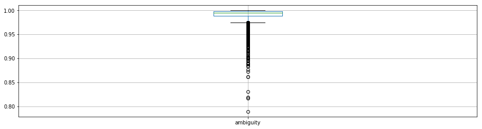
Clearly, Lowe’s suggested 0.8 ratio is going to remove almost all of the data. The 0.95 threshold looks attractive as it is below the lower quartile break.

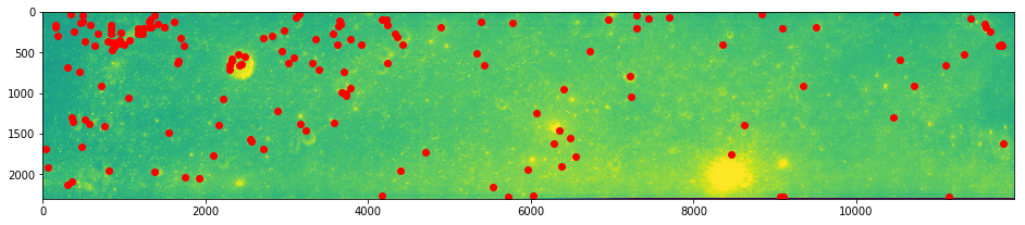
ksub = matches[matches.ambiguity <= 0.95]

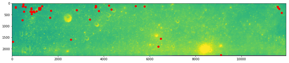
# And plot
imshow(arr0)
plot(ksub.x, ksub.y, 'ro')
show()
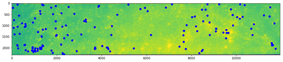
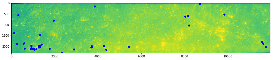
imshow(arr1)
plot(ksub.match_xpos, ksub.match_ypos, 'bo')
show()

Score

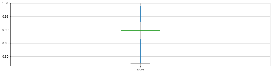
ksub.boxplot(column='score')
ksub.score.describe()

count    163.000000
mean       0.898343
std        0.048708
min        0.775125
25%        0.866216
50%        0.897366
75%        0.929772
max        0.989991
Name: score, dtype: float64

kss = ksub[ksub.score >= 0.925310]
imshow(arr0)
plot(kss.x, kss.y, 'ro')
show()
imshow(arr1)
plot(kss.match_xpos, kss.match_ypos, 'bo')
show()

The combined reduction due to ambiguity and score winnowing has generated what looks like a relatively good starting point for more robust outlier detection methods.